Rotate

To rotate a model, we can't just add or multiply. Instead we apply some trigonometric operations to each position. In two dimensions, the amount of rotation is determined by an angle—which is a scalar rather than a vector. By mathematical convention, a positive angle rotates the model counter-clockwise.

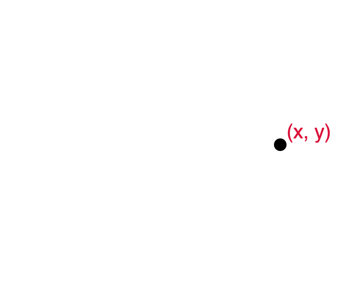
Figuring out the trigonometric operations is easier if we represent each position not in Cartesian coordinates but in polar coordinates. In Cartesian coordinates, a position is an x- and y-offset. In polar coordinates, a position is a radius and an angle. Any given position can be expressed in both systems:

Coordinates in one system can be converted to the other. Step through the following sequence to see how Cartesian coordinates and polar coordinates relate:

1. A point $\mathbf{p}$ has Cartesian coordinates $\begin{bmatrix}x & y\end{bmatrix}$.
2. Elsewhere on the grid is the origin.
3. The Euclidean distance between the origin and $\mathbf{p}$ is $r$.
4. Point $\mathbf{p}$ is situated on the perimeter of a circle centered on the origin and of radius $r$.
5. The horizontal distance between $\mathbf{p}$ and the origin is $x$.
6. The vertical distance between $\mathbf{p}$ and the origin is $y$.
7. The three distances $r$, $x$, and $y$ are the side lengths of a right-triangle.
8. The angle between the x-axis and point $\mathbf{p}$ is $a$. Point $\mathbf{p}$ is expressed in polar coordinates as $(r, a)$.

⭠ ⭢

The trigonometric identities you learned earlier in life tell us these facts about how the sides and angle relate:

We solve for \(x\) and \(y\) to get the equations that turn polar coordinates into Cartesian coordinates:

Hold onto these equations. We'll recall them in a moment.

Here then is the problem of rotation. We have an existing point \(\mathbf{p}\), and we want to rotate it \(b\) radians to compute the rotated point \(\mathbf{p}'\). In polar coordinates, \(\mathbf{p}'\) is a lot like \(\mathbf{p}\). It's just rotated a bit more:

Now we apply the polar-to-Cartesian formulas from above to find the rotated point's Cartesian coordinates:

Those cosine and sine of sums may be expanded with help from these trigonometric sum identities that you may not remember:

After expanding the sums, we arrive at these seemingly unhelpful equations:

But wait. We can simplify a bit. First we distribute \(r\):

Do you see that \(r \cos a\)? You know what that is? That's \(x\). We saw it earlier as the Cartesian x-coordinate of unrotated \(\mathbf{p}\). And \(r \sin a\) is \(y\). We substitute these in:

And those are our equations for rotating. We combine the x- and y-coordinates of the unrotated position \(\mathbf{p}\) together with some trigonometric functions of the angle of rotation. Observe that we never actually convert to polar coordinates in these final equations. We just used polar coordinates to derive them.

This vertex shader rotates the incoming position property by the uniform radians:

uniform float radians;
in vec3 position;

void main() {
  gl_Position = vec4(
    position.x * cos(radians) - position.y * sin(radians),
    position.x * sin(radians) + position.y * cos(radians),
    position.z,
    1.0
  );
}

uniform float radians;
in vec3 position;

void main() {
  gl_Position = vec4(
    position.x * cos(radians) - position.y * sin(radians),
    position.x * sin(radians) + position.y * cos(radians),
    position.z,
    1.0
  );
}

On the CPU side, we supply a value for radians:

shader.setUniform1f('radians', 0.1);

shader.setUniform1f('radians', 0.1);

There's no vectorized operation for rotation like there is for translation and scaling—at least not a simple one. In the next chapter we'll learn how all three transformations can be expressed as matrix operations, which will make them fast to compute and easier to combine.

Summary

Vertices are the atoms of computer graphics, but we almost always bond them together into triangles. Any surface can be expressed as a collection of triangles. We may represent each triangle independently in a sequence of vertex triplets, or we can make a quilt of shared vertices by explicitly grouping them in an index buffer. Properties are defined only at a triangle's vertices, but the values within are computed by interpolating. We can also define uniform data that is shared across all vertices and triangles. Surfaces are moved, stretched, and spun using the three standard transformations: translate, scale, and rotate. The parameters of these transformations are set as uniforms and applied in the vertex shader.