Gradient Noise

In the 1980s, Ken Perlin proposed an alternative noise algorithm that does not exhibit the artifacts of value noise. Perlin had been hired by the Mathematical Applications Group, Inc. (MAGI), to work on the movie Tron. The movie was a technical feat for the time, but Perlin said this of his experience:

Working on TRON was a blast, but on some level I was frustrated by the fact that everything looked machine-like. In fact, that became the "look" associated with MAGI in the wake of TRON. So I got to work trying to help us break out of the "machine-look ghetto."

Perlin published his noise algorithm in 1985. It was adopted by many artists in the motion picture industry, and Perlin went on to win an Academy Award for the algorithm in 1997.

Instead of generating random scalars at every lattice point, Perlin's algorithm generates random vectors. These vectors describe the slope of some random pattern through the space. Such vectors are called gradients, and Perlin's noise is therefore called gradient noise. The noise values themselves are not random; they are computed to fit the shape of the random gradients.

Let's implement our own Perlin 2D noise generator. There are many tutorials on the web explaining Perlin noise. There are several reasons for their abundance: the algorithm is sophisticated enough to need explanation, Perlin himself published several different versions of the algorithm, and many explanations focus on optimizations. Our discussion here will be confined to a simpler unoptimized implementation.

Random Gradients

First we need a grid of random gradients pointing in all directions. We could generate a random gradient by choosing a random point within a unit square, like this:

function randomGradient
  x = random(-1, 1)
  y = random(-1, 1)
  return new Vector2(x, y).normalize

function randomGradient
  x = random(-1, 1)
  y = random(-1, 1)
  return new Vector2(x, y).normalize

There's a problem with this approach, however. We are more likely to choose a point on the square's diagonal than in a cardinal direction because a square's diagonals are longer than its sides. The gradients will not be uniformly distributed. To avoid this bias, we express the gradient in polar coordinates—as a radius and angle. The radius is 1 since the gradient should have unit length. The angle we draw randomly from $[0, 2\pi)$. Then we convert the polar coordinates to Cartesian coordinates to form a vector:

function randomGradient
  angle = random(0, 2 * pi)
  x = cos angle
  y = sin angle
  return new Vector2(x, y)

function randomGradient
  angle = random(0, 2 * pi)
  x = cos angle
  y = sin angle
  return new Vector2(x, y)

This pseudocode produces a uniformly distributed 2D array of gradients:

gradients = new grid of dimensions (width, height)
for each row r
  for each column c
    gradients[c, r] = randomGradient

gradients = new grid of dimensions (width, height)
for each row r
  for each column c
    gradients[c, r] = randomGradient

The result is a field of vectors that looks something like this:

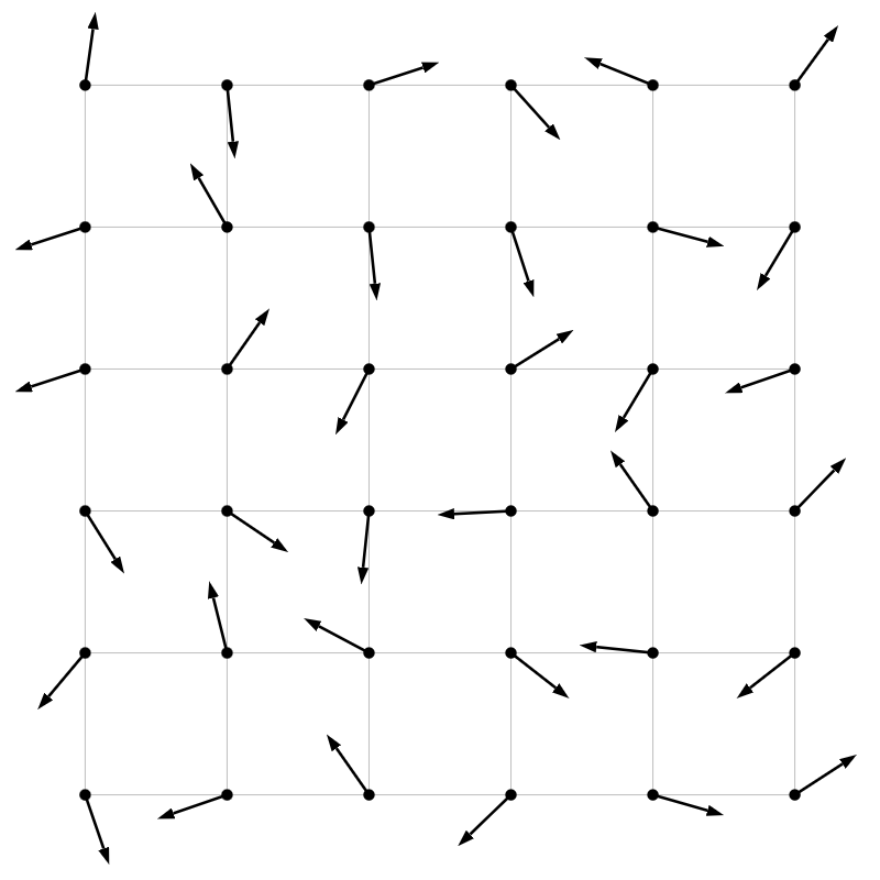
We want to create this field of gradients just once and use it over and over again for all of our noise lookups. The exact resolution is not so important. Even if it's small, we'll make the gradients tile infinitely across the whole 2D plane.

Interpolation

The second ingredient to Perlin noise is a function that generates a random but coherent scalar value at an arbitrary position $p$. We need to find the fraction of $p$ within its surrounding cell of four neighbors, just as we did in the blerp routine in the Field2 class. Additionally, we need the coordinates of the four lattice points. All these values can be derived from the floor and ceiling of $p$:

function noise(p)
  floor = floor of p
  ceiling = floor + [1, 1]
  fraction = p - floor

function noise(p)
  floor = floor of p
  ceiling = floor + [1, 1]
  fraction = p - floor

The position $p$ may lie outside the gradient grid, so we need to wrap it to be in bounds. We often use the % operator for wrapping.

If the coordinates are positive, the % operator wraps them back in bounds just as we'd expect. But % doesn't wrap negative numbers in the same way. We use this more robust formula:

function wrap(x, period)
  return (x % period + period) % period

function wrap(x, period)
  return (x % period + period) % period

Suppose period is 10. The x % period operation gives us a value in [-9, 9]. Adding 10 moves us out of the negatives into [1, 19]. The second % wraps us back into [0, 9].

We now wrap the floor and ceiling so we can use them as indices in the gradients array:

function noise(p)
  // ...
  wrappedFloor = wrap floor into gradient dimensions
  wrappedCeiling = wrap ceiling into gradient dimensions

function noise(p)
  // ...
  wrappedFloor = wrap floor into gradient dimensions
  wrappedCeiling = wrap ceiling into gradient dimensions

The four neighboring gradients around $p$ shape the organic surface within the cell. We use the wrapped floor and ceiling to grab the gradients at the four corners:

function noise(p)
  // ...
  gradient00 = gradients[wrappedFloor.x, wrappedFloor.y]
  gradient10 = gradients[wrappedCeiling.x, wrappedFloor.y]
  gradient01 = gradients[wrappedFloor.x, wrappedCeiling.y]
  gradient11 = gradients[wrappedCeiling.x, wrappedCeiling.y]

function noise(p)
  // ...
  gradient00 = gradients[wrappedFloor.x, wrappedFloor.y]
  gradient10 = gradients[wrappedCeiling.x, wrappedFloor.y]
  gradient01 = gradients[wrappedFloor.x, wrappedCeiling.y]
  gradient11 = gradients[wrappedCeiling.x, wrappedCeiling.y]

Somehow we need to turn $p$ and the four gradients into a random value that varies smoothly within the cell. Perlin's idea was to find vectors from the four corners to $p$:

function noise(p)
  // ...
  diff00 = p - floor
  diff10 = p - [ceiling.x, floor.y]
  diff01 = p - [floor.x, ceiling.y]
  diff11 = p - ceiling

function noise(p)
  // ...
  diff00 = p - floor
  diff10 = p - [ceiling.x, floor.y]
  diff01 = p - [floor.x, ceiling.y]
  diff11 = p - ceiling

And then dot each with the corresponding gradient vector:

function noise(p)
  // ...
  dot00 = dot(gradient00, diff00)
  dot10 = dot(gradient10, diff10)
  dot01 = dot(gradient01, diff01)
  dot11 = dot(gradient11, diff11)

function noise(p)
  // ...
  dot00 = dot(gradient00, diff00)
  dot10 = dot(gradient10, diff10)
  dot01 = dot(gradient01, diff01)
  dot11 = dot(gradient11, diff11)

Explore the dot product calculation in the renderer below. It shows a single cell with its four surrounding gradients. When you move the mouse within the cell, the difference vectors point to the location of the noise value. The dot products indicate the alignment between the gradients and difference vectors.

These four dot products describe how much $p$ aligns with the gradient vectors. We've got four numbers and want to reduce them down to one. Perlin suggested blerping them based on the fractional position of $p$:

function noise(p)
  // ...
  dot0 = lerp(dot00, dot10, fraction.x)
  dot1 = lerp(dot01, dot11, fraction.x)
  dot = lerp(dot0, dot1, fraction.y)
  return dot

function noise(p)
  // ...
  dot0 = lerp(dot00, dot10, fraction.x)
  dot1 = lerp(dot01, dot11, fraction.x)
  dot = lerp(dot0, dot1, fraction.y)
  return dot

Enable interpolation in the renderer and watch how the noise value smoothly changes as you move the mouse.

The noise function produces only a single scalar value. To generate a complete field, we call it repeatedly across a grid:

function noiseField(width, height, scale)
  field = new field of dimensions (width, height)
  for each row r
    for each column c
      field[c, r] = noise((c, r) * scale)
  return field

function noiseField(width, height, scale)
  field = new field of dimensions (width, height)
  for each row r
    for each column c
      field[c, r] = noise((c, r) * scale)
  return field

The column and row indices are scaled, which zooms into the noise. The scale factor should be a number in $[0, 1]$.

With this much of the algorithm implemented, we are able to produce noise textures that look like this:

This noise might be smooth, but it's too dark.

Normalize

The noise is too dark because the computed noise values never reach 1. That would happen only if all the vectors were in alignment, and that's simply not possible. A workaround is to normalize the values to the range $[0, 1]$. We range-map the values from their native range $[\mathrm{min}, \mathrm{max}]$ to $[0, 1]$ with this arithmetic gauntlet:

$$\begin{align} [\mathrm{min}, \mathrm{max}] \xrightarrow{-~\mathrm{min}} [0, \mathrm{max} - \mathrm{min}] \xrightarrow{\div~(\mathrm{max} - \mathrm{min})} [0, 1] \end{align}$$

Enable normalization in this renderer to see the improvement:

There's more contrast, but there are also visible squares.

Weight Smoothing

The discontinuities appear at cell boundaries. Within a cell, the random values are perfectly smooth. But when we transition to a neighboring cell, we might switch to a very different curve. The fix is to run the blending weights through a smoothing function like this one:

$$\mathrm{smooth}(x) = 6x^5 - 15x^4 + 10x^3$$

This plot shows the raw weight in red and the smoothed weight in blue:

The smoothed weight has a derivative of 0 at the cell boundaries, which flattens the discontinuities between neighboring cells' curves. We apply the smoothing function to our fraction vector right before lerping:

function noise(p)
  // ...
  smoothFraction = [smooth(fraction.x), smooth(fraction.y)]
  dot0 = lerp(dot00, dot10, smoothFraction.x)
  dot1 = lerp(dot01, dot11, smoothFraction.x)
  dot = lerp(dot0, dot1, smoothFraction.y)
  // ...

function noise(p)
  // ...
  smoothFraction = [smooth(fraction.x), smooth(fraction.y)]
  dot0 = lerp(dot00, dot10, smoothFraction.x)
  dot1 = lerp(dot01, dot11, smoothFraction.x)
  dot = lerp(dot0, dot1, smoothFraction.y)
  // ...

Enable normalization and smoothing in this renderer to see a much nicer specimen of noise:

This noise is looking much better.

Octaves

With normalization and smoothing enabled, bump the resolution of the noise up to 200×200. The result is definitely better than white noise, but the texture lacks features. It looks like worms crawled across some loose soil. We fix this by blending octaves of noise together. Just as with pyramids of value noise, big features must be assigned more weight and fine details less weight.

How do we determine these weights? Let's say the first octave has weight $\frac{1}{d}$, where $d$ is some denominator that we haven't figured out yet, and that there are $c$ octaves. Each successive weight is twice its predecessor, which gives us this geometric sequence of weights:

$$\frac{1}{d}, \frac{2}{d}, \frac{4}{d}, \frac{8}{d} \ldots \frac{2^{c - 1}}{d}$$

We want the weights to sum to 1 to keep the noise normalized. This constraint helps us solve for the unknown denominator:

$$\begin{align} \frac{1}{d} + \frac{2}{d} + \frac{4}{d} + \frac{8}{d} + \ldots + \frac{2^{c - 1}}{d} &= 1 \\ \frac{1 + 2 + 4 + 8 + \ldots + 2^{c - 1}}{d} &= 1 \\ 1 + 2 + 4 + 8 + \ldots + 2^{c - 1} &= d \\ \end{align}$$

Denominator $d$ is a sum of a sequence of powers of 2. What do you notice about these sums of the first several such sequences?

$$\begin{align} 1 &= 1 \\ 1 + 2 &= 3 \\ 1 + 2 + 4 &= 7 \\ 1 + 2 + 4 + 8 &= 15 \\ 1 + 2 + 4 + 8 + 16 &= 31 \\ 1 + 2 + 4 + 8 + 16 + 32 &= 63 \\ \end{align}$$

The sums are just one less than the next power of 2. In general, we compute $d$ with this shortcut:

$$\begin{align} d &= \sum_{i = 0}^{c - 1} 2^i \\ &= 2^c - 1 \\ \end{align}$$

Raising 2 to the power $n$ is equivalent to left-shifting 1 by $n$. We use this fact to implement the fractalNoise function, which loops through the octaves, calls upon the regular noise function to produce each octave's noise value, and computes a weighted sum of all the values:

fractalNoise(p, octaveCount) {
  sum = 0
  denominator = (1 << octaveCount) - 1
  for each octave i
    weight = (1 << i) / denominator
    sum += noise(p / (1 << i)) * weight
  return sum

fractalNoise(p, octaveCount) {
  sum = 0
  denominator = (1 << octaveCount) - 1
  for each octave i
    weight = (1 << i) / denominator
    sum += noise(p / (1 << i)) * weight
  return sum

Position $p$ is scaled down with each successive octave to ensure different positions are used at each octave.

The renderer below has an updated noiseField function that calls fractalNoise instead of noise. Bump up the number of octaves to produce some very fine noise:

This noise is music.

← Value Noise Heightmaps →

How to 3D